NoSpherA2 Properties
This part is a utility for plotting and visualizing the results of NoSpherA2. Select desired resolution of the grid to be calculated and properties to evaluate and click calculate to start the beackground generation of grids. When done the calcualted fields will become available from the dropdown to show maps. Sometimes it is necessary to open and close the Properties dropdown in order to show all avalable maps.
The reading of maps might take some time and Olex2 might become irresponsive, please be patient.
So far the calculation can only happen in the unit cell and on the wavefunction in the folder. If you need an updated wavefunction (e.g. due to moved atoms or different spin state) hit the update .tsc file button.
The calcualtion will be carried out for your selected unit used in the wavefunction calculation procedure. If it is reachign outside the unit cell the contribution to the neighbouring unit cell will also appear in the unit cell translated, which can lead to “cutoff” effects, if you have a large radius selected.
The obtainable plots depend on your wavefunction calculated. Please make sure it is reasonbale.
If you use multiple CPUs the progress bar might behave in non-linear ways, this is due to the computations being executed in parallel and all CPUs being able to report progress. Some parts of the calculation might be faster than others.
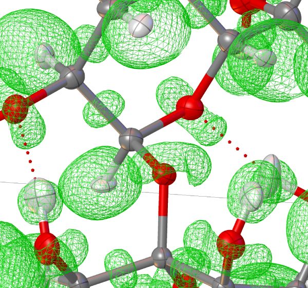
Lap(lacian of the eectron density)
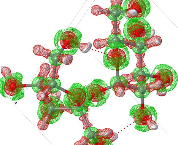
Laplacian (second derivative) of the electron density. This grid shows regions of electron accumulation (negative values) and elecrton depletion (positive values), as it is the curvature of the electron density. Usefull to understand polarisation of bonds, position of lone-pairs etc.
Sometimes it is also very usefull to look at the laplacian map in 2D-planes to udnerstand the shape of the electron accumulation (e.g. lone-pairs or bonds).
These plots can tell a lot about reactivity and chemical behaviour of individual functional groups.
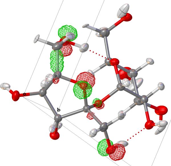
ELI
Calculates the Electron Localizability Indicater. This function in summary describes the volume needed to find a different electron to the one at position r. This measure of localization very well correpsonods with chemically intuitive feautures like lone-pairs, bonds etc. The shape of isosurfaces is usually a nice indicator for bonding situations. In Olex2 the ELI-D of same spin alpha electrons is used.
A nice overview of all kinds of indicators developed by the original authors and their application is given on this website:
- Electron Localizability Indicators
 Paper
Paper
ELF
Calcuales the arbitrarily scaled Electron Localisation Function. This function is scaled between 0 and 1. There is no general rule how to select isovalues. Only included for legacy reasons. In general it is recommended to use ELI.
ESP
Calculation of the total electrostatic potential. This is a complex caluclation, since the potential V is an integral over the whole wavefunction.
This integral yields the potential at each point in space due to all other electrons in the wavefunction which a test particle would experience, therefore the calculation of ESP does not scale with the third power of resolution of the grid, but also cubically with the number of basis functions and electrons, which makes it really time consuming.
If you decide to cancel the job all cubes of the other calculations will be saved before starting ESP calculation, so you can restart only the ESP step.
MO
Lets you calculate the isosurfaces of individual MOs of your .wfn file. select individual MOs or “All MOs” to calcualte all in one go. The selected number will also be the one used for plotting.
HDEF
Hirshfeld Deformation Density of atoms will be calculated in a .cube file for each atom. Mostly for testing and benchamrking. Not suitable for routine use.
Radius
Select how far away a point in the grid will still be evaluated from any atom in the wavefunction. Smaller values make the calculation faster, as more points can be skipped, but might truncate the maps.
Res(olution)
Defines the resolution the calculated grid should have. Keep in mind that the ressource demand of the calculation rises cubically.
Calculate
Start the calculaton of selected fields using NoSpherA2.
Map
Selects which map is to be displayed. Only shows maps, which are already available. if a calculated map is not shown close and open the Properties window once. If that does not help try chekcing if all cubes are found. If there is none available try to calculate a new wavefunction or check for LIST 3 or 6 in the .ins file, as a .fcf file with phases is needed.
Toggle Map
Shows/Hides Map
View
Selects whaype of mapis to be displayed. Choices include:
- plane - 2D
- plane + contour 2D
- wire - 3D
- surface - 3D
- points - 3D
Edit Style
Edits the colour of the various map surfaces.
Level
When a 3D map is displayed the slider bar enables you to adjust the isovalue and therefore detail shown in the map. Some values are “locked” since they would simply show too many things on screen.
Min
This will define the minimum value of your 2D map. The slider works in quarter-integer values but also accepts manual input in the text-box next to it.
Step
This will define the step size of your 2D map between two contours/colours. As with Min this slider has pre-defined slider values, but also manual input will work.
Depth
This slider controls the depth of the 2D-plane “into” the screen. If the value is negative the map will go “behind” the model, positive will move it to the front.
If you select atoms and click on the Depth button the map will be aligned so the map is in plane with these selected atoms.
Size
Size will control the size of the plotted 2D-plane. Bigger values will decrease the visual size, but will increase the resultion of the map.